Patrick AMAR

Bioinfo group, LISN, Univ. Paris Saclay, UMR 9015 CNRS
Synthetic & Systems Biology group, Sys2diag UMR 9005 CNRS, ALCEN

Quick overview

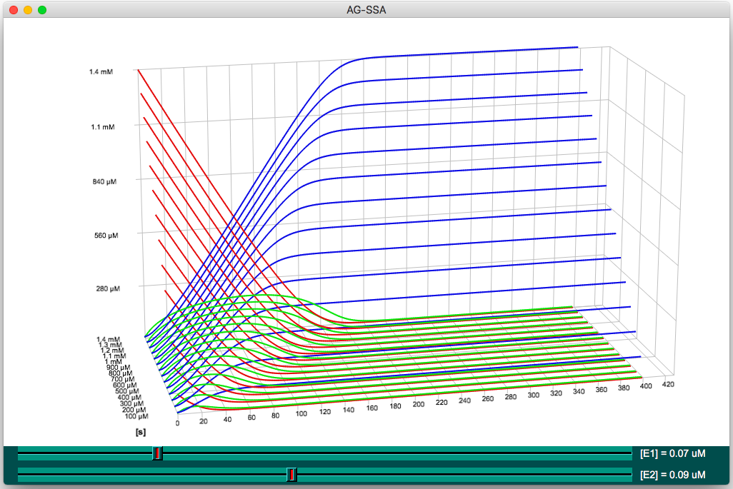
AG-SSA is a massively parallel simulation tool that run on both multicore CPU and on GPU devices. The algorithm used can be switched to perform either discrete stochastic, or continuous deterministic simulations. The input is an enzymatic reactions system, with kinetics and initial ranges of concentration values. The combination of initial values lead to many independent simulations of the same model that will run in parallel. The output is the time trajectory of selected molecular species. They can be plotted with the companion software Curves3D.

For example, this simple model of the cascade of two enzymatic reactions is simulated by 1400 parallel threads. There are 14 different concentration values of the initial substrate s, 10 concentrations of enzyme E1, and 10 concentrations of enzyme E2. The model is simulated for 400 s (virtual time) and exports the trajectories of the initial s, intermediate p and final q products.

	[E1] = 0.05 uM -> 0.15 uM : 0.01 uM;
	[E2] = 0.01 uM -> 0.2 uM : 0.02 uM;

	[s] = 0.1 mM -> 1.5 mM : 0.1 mM;

	duration = 400;
	display (p, s, q);

	# E1 and E2 have the same kinetics: Km = 0.1 mM and Kcat = 150

	E1 : s -> p | 0.1 mM - 150;
	E2 : p -> q | 0.1 mM - 150;

The 1400 stochastic simulations took 4.01 s on a GTX 1050 GPU vs 48.61 s on a 4-cores Intel Core I5 CPU and 177.9 s for the sequential version on the same CPU.

The images below are snapshots of the Curves3D software displaying the output of these simulations under two different viewing angles. Each curve represents the trajectory of a set of metabolites (substrate s in red, intermediate product p in green, final product q in blue) one set for each of the 14 concentrations of the s input metabolite. The scrollbars select the concentrations of enzymes E1 and E2, displaying the corresponding sets of curves.

Windows Version	(February 7, 2023) AG-SSA	/  Curves3D
Linux Version	(February 7, 2023) AG-SSA	/  Curves3D
Mac OS X (x86_64) Version	(February 7, 2023) AG-SSA	/  Curves3D
Linux (CUDA) Version	(February 7, 2023) AG-SSA

 

Installation

On Linux and MacOS X copy the executable files ag-ssah, ag-ssa and Curves3D (or ag-ssah-osx and curves3D-osx) into a directory listed in the PATH environment variable and make them executable (chmod 755 ag-ssah Curves3D).

On Windows copy the executable files ag-ssah.exe and Curves3D.exe into the C:\Windows\System32 folder.

AG-SSA Reference manual

AG-SSA (GPU version) and AG-SSAH (CPU version) are launched from the command line. Each version have common and distinctive options.

• -v(erbose) displays on stderr the initial number of copies of each reactant, and the model translated to basic 1 or 2 reactants interactions.
• -d(eterministic)
  use the continuous deterministic version of the simulation algorithm.
• -o(ut) output-file
  saves the (gzipped) simulations results into output-file. If output-file is '-' stdout is used, so it can be piped to the input of Curves3D. The default output file is data.gz.
• -s(equential) (CPU version only)
  use only one thread.
• -npt (CPU version only)
  displays the number of cores of the CPU.
• -g(pu-verbose) (GPU version only)
  displays infos about the GPU device, along with the number of threads per block, the number of blocks per grid, and the size of the shared memory used to simulate the model. For example, using the cascade model shown above:

  Device 0: "GeForce GTX 1050 Ti", 6 x 128 = 768 CUDA Cores. Warpsize = 32
  Threads per block: 32, Blocks per Grid: 44, Shared Memory: 1152
  n_threads = 1400, n_species = 7, n_reactions = 6
  Simulated time: 400 s, Simulation time: 4.04 s

The input file specifies (in any order) the enzymatic reactions along with their kinetics, the initial concentrations of the reactants, the duration of the simulation and which species should be displayed (by Curve3D).
The syntax is simple and intuitive:

		E : s1 + s2 -> p1 + p2 | 1 mM, 300 uM - 200;

first the enzyme that catalyzes the reaction, the reaction itself, then the kinetics K_m (as many as there are substrates) and K_cat. These fields are separated by punctuations. The + operator is used to specify multiple substrates or products.

Enzymes can be inhibited by metabolites. To specify that inh inhibits E with the affinity K_i = 30 uM:

		E : inh | 30 uM;

The concentrations can be given in micromolar (uM) or in millimolar (mM). The default initial concentrations are 0 unless specified with:

		[E] = 0.1 uM;
		[s1] = 0.8 uM, 1 uM, 5 uM, 50 uM;
		[s2] = 30 uM -> 50 uM : 2.5 uM;

The enzyme concentration is the fixed value 0.1 micromolar. The concentration of the s1 substrate will take the successive four values 0.8, 1, 5, and 50 micromolar in four series of simulations. The concentration of the s2 substrate will take the successive nine values from 30 uM up to 50 uM with a 2.5 uM step, leading to 4*9 = 36 simulations that will run in parallel.

The varying concentrations of two, or more, species can be linked. For example, when

		linked (s1, s2);

The duration of the simulation (in seconds) is specified with:

		duration = 400;

		display (s1, s2 #008000, p1 #000);

In this example s1 will be drawn in red, s2 in dark green, and p1 in black.

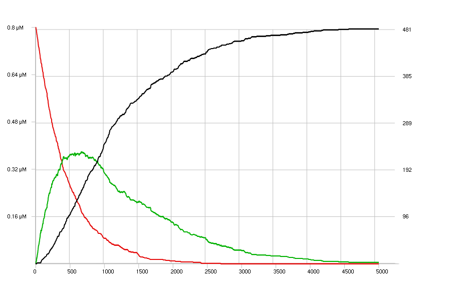
The images below show the simulations of the sample model, with only one set of very low concentrations:

		[s] = 0.8 uM;
		[E1] = 0.05 uM;
		[E2] = 0.07 uM;

		duration = 5000;
		display (s, p #00b000, q #000);

		E1 : s -> p | 2 mM - 100;
		E2 : p -> q | 5 mM - 90;

The top view shows a discrete stochastic simulation, and the bottom view a continuous deterministic simulation of this model. The Curves3D viewer has been set to display a flat view of the curves; The concentrations are shown on the left Y-axis and the corresponding number of molecules on the right Y-axis.

discrete stochastic simulation

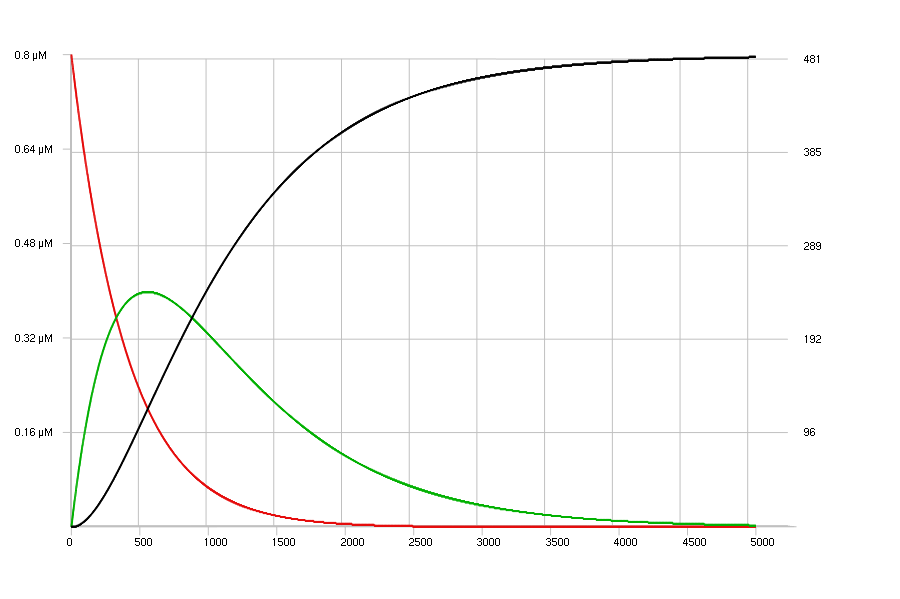
continuous deterministic simulation

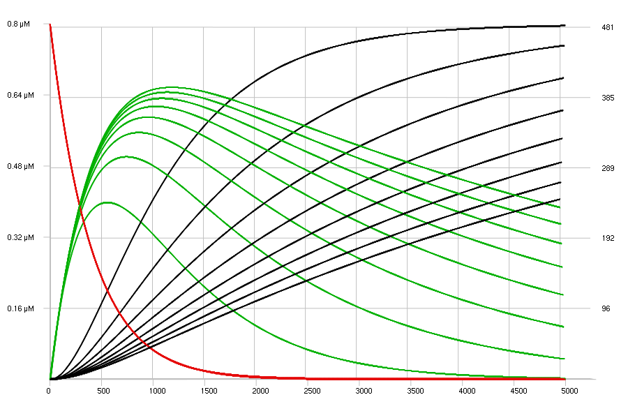
Inhibition of E2 has been added to show the effect of various concentrations of inhibitor i, from 0 to 210 uM.

		[i] = 0 uM -> 210 uM : 30 uM;
		E2 : i | 30 uM;

The results are shown below, using again a 2D flat view.

continuous deterministic simulation, with E2 inhibited

Curves3D Reference manual

Curves3D is used to interactively display the results of the simulations output by AG-SSA.
The trajectories of the species, which have its set of varying concentrations defined last in the model file, are plotted with curves drawn along the Z-axis. The varying concentrations for the other species are chosen with the scrollbars displayed at the bottom of the window.

In the first examples (top of the page), a set of curves is plotted along the Z-axis for each concentration of the s species. The two scrollbars allows the user to select the concentration of enzyme E1 and E2.

input-file is either a gzipped (or not) file, or '-' for stdin.

• -r(everse video) the curves are displayed on a black background instead of a white background.
• -d(elete input-file) the input file is removed just after being read. This option is used for temporary files.

Mouse commands

• Left drag rotates the curves around the center of the bounding box.
• Right drag translates the displayed curves laterally or vertically.
• The wheel zooms in or out the display.
• With the Shift keyboard modifier pressed, the wheel changes the depth of the view. The display along the Z-axis can be then flattened or expanded.
• With the Ctrl keyboard modifier pressed, the wheel changes the Y-axis scale (concentrations).